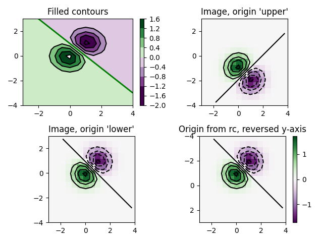
Image de contour #

Testez des combinaisons de contours, de contours remplis et de tracés d'images. Pour l'étiquetage de contour, voir également l' exemple de démonstration de contour .

Dans cette démonstration, l'accent est mis sur la façon de faire en sorte que les contours s'alignent correctement sur les images et sur la façon de les orienter tous les deux comme vous le souhaitez. En particulier, notez l'utilisation des arguments de mots-clés "origin" et "extent" pour imshow et contour.

import matplotlib.pyplot as plt
import numpy as np
from matplotlib import cm

# Default delta is large because that makes it fast, and it illustrates
# the correct registration between image and contours.
delta = 0.5

extent = (-3, 4, -4, 3)

x = np.arange(-3.0, 4.001, delta)
y = np.arange(-4.0, 3.001, delta)
X, Y = np.meshgrid(x, y)
Z1 = np.exp(-X**2 - Y**2)
Z2 = np.exp(-(X - 1)**2 - (Y - 1)**2)
Z = (Z1 - Z2) * 2

# Boost the upper limit to avoid truncation errors.
levels = np.arange(-2.0, 1.601, 0.4)

norm = cm.colors.Normalize(vmax=abs(Z).max(), vmin=-abs(Z).max())
cmap = cm.PRGn

fig, _axs = plt.subplots(nrows=2, ncols=2)
fig.subplots_adjust(hspace=0.3)
axs = _axs.flatten()

cset1 = axs[0].contourf(X, Y, Z, levels, norm=norm,
                        cmap=cmap.resampled(len(levels) - 1))
# It is not necessary, but for the colormap, we need only the
# number of levels minus 1.  To avoid discretization error, use
# either this number or a large number such as the default (256).

# If we want lines as well as filled regions, we need to call
# contour separately; don't try to change the edgecolor or edgewidth
# of the polygons in the collections returned by contourf.
# Use levels output from previous call to guarantee they are the same.

cset2 = axs[0].contour(X, Y, Z, cset1.levels, colors='k')

# We don't really need dashed contour lines to indicate negative
# regions, so let's turn them off.

for c in cset2.collections:
    c.set_linestyle('solid')

# It is easier here to make a separate call to contour than
# to set up an array of colors and linewidths.
# We are making a thick green line as a zero contour.
# Specify the zero level as a tuple with only 0 in it.

cset3 = axs[0].contour(X, Y, Z, (0,), colors='g', linewidths=2)
axs[0].set_title('Filled contours')
fig.colorbar(cset1, ax=axs[0])


axs[1].imshow(Z, extent=extent, cmap=cmap, norm=norm)
axs[1].contour(Z, levels, colors='k', origin='upper', extent=extent)
axs[1].set_title("Image, origin 'upper'")

axs[2].imshow(Z, origin='lower', extent=extent, cmap=cmap, norm=norm)
axs[2].contour(Z, levels, colors='k', origin='lower', extent=extent)
axs[2].set_title("Image, origin 'lower'")

# We will use the interpolation "nearest" here to show the actual
# image pixels.
# Note that the contour lines don't extend to the edge of the box.
# This is intentional. The Z values are defined at the center of each
# image pixel (each color block on the following subplot), so the
# domain that is contoured does not extend beyond these pixel centers.
im = axs[3].imshow(Z, interpolation='nearest', extent=extent,
                   cmap=cmap, norm=norm)
axs[3].contour(Z, levels, colors='k', origin='image', extent=extent)
ylim = axs[3].get_ylim()
axs[3].set_ylim(ylim[::-1])
axs[3].set_title("Origin from rc, reversed y-axis")
fig.colorbar(im, ax=axs[3])

fig.tight_layout()
plt.show()

Contours remplis, Image, origine 'supérieur', Image, origine 'inférieur', Origine de rc, axe y inversé

Références

L'utilisation des fonctions, méthodes, classes et modules suivants est illustrée dans cet exemple :

Galerie générée par Sphinx-Gallery