Noter
Cliquez ici pour télécharger l'exemple de code complet
Annotation de tracés #
Les exemples suivants montrent comment il est possible d'annoter des tracés dans Matplotlib. Cela comprend la mise en évidence de points d'intérêt spécifiques et l'utilisation de divers outils visuels pour attirer l'attention sur ce point. Pour une description plus complète et approfondie des outils d'annotation et de texte dans Matplotlib, consultez le tutoriel sur l'annotation .
import matplotlib.pyplot as plt
from matplotlib.patches import Ellipse
import numpy as np
from matplotlib.text import OffsetFrom
Spécification des points de texte et des points d'annotation #
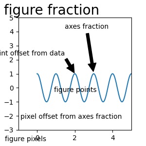
Vous devez spécifier un point d'annotation pour annoter ce point. De plus, vous pouvez spécifier un point de texte pour l'emplacement du texte de cette annotation. Facultativement, vous pouvez spécifier le système de coordonnées de xy et xytext avec l'une des chaînes suivantes pour xycoords
et textcoords (la valeur par défaut est 'data') :xy=(x, y)xytext=(x, y)
'figure points'   : points from the lower left corner of the figure
'figure pixels'   : pixels from the lower left corner of the figure
'figure fraction' : (0, 0) is lower left of figure and (1, 1) is upper right
'axes points'     : points from lower left corner of axes
'axes pixels'     : pixels from lower left corner of axes
'axes fraction'   : (0, 0) is lower left of axes and (1, 1) is upper right
'offset points'   : Specify an offset (in points) from the xy value
'offset pixels'   : Specify an offset (in pixels) from the xy value
'data'            : use the axes data coordinate system
Remarque : pour les systèmes de coordonnées physiques (points ou pixels), l'origine est le (en bas, à gauche) de la figure ou des axes.
Facultativement, vous pouvez spécifier les propriétés de la flèche qui dessine et la flèche du texte au point annoté en donnant un dictionnaire des propriétés de la flèche
Les clés valides sont :
width : the width of the arrow in points
frac  : the fraction of the arrow length occupied by the head
headwidth : the width of the base of the arrow head in points
shrink : move the tip and base some percent away from the
         annotated point and text
any key for matplotlib.patches.polygon  (e.g., facecolor)
# Create our figure and data we'll use for plotting
fig, ax = plt.subplots(figsize=(3, 3))

t = np.arange(0.0, 5.0, 0.01)
s = np.cos(2*np.pi*t)

# Plot a line and add some simple annotations
line, = ax.plot(t, s)
ax.annotate('figure pixels',
            xy=(10, 10), xycoords='figure pixels')
ax.annotate('figure points',
            xy=(80, 80), xycoords='figure points')
ax.annotate('figure fraction',
            xy=(.025, .975), xycoords='figure fraction',
            horizontalalignment='left', verticalalignment='top',
            fontsize=20)

# The following examples show off how these arrows are drawn.

ax.annotate('point offset from data',
            xy=(2, 1), xycoords='data',
            xytext=(-15, 25), textcoords='offset points',
            arrowprops=dict(facecolor='black', shrink=0.05),
            horizontalalignment='right', verticalalignment='bottom')

ax.annotate('axes fraction',
            xy=(3, 1), xycoords='data',
            xytext=(0.8, 0.95), textcoords='axes fraction',
            arrowprops=dict(facecolor='black', shrink=0.05),
            horizontalalignment='right', verticalalignment='top')

# You may also use negative points or pixels to specify from (right, top).
# E.g., (-10, 10) is 10 points to the left of the right side of the axes and 10
# points above the bottom

ax.annotate('pixel offset from axes fraction',
            xy=(1, 0), xycoords='axes fraction',
            xytext=(-20, 20), textcoords='offset pixels',
            horizontalalignment='right',
            verticalalignment='bottom')

ax.set(xlim=(-1, 5), ylim=(-3, 5))
[(-1.0, 5.0), (-3.0, 5.0)]
Utilisation de plusieurs systèmes de coordonnées et types d'axes #
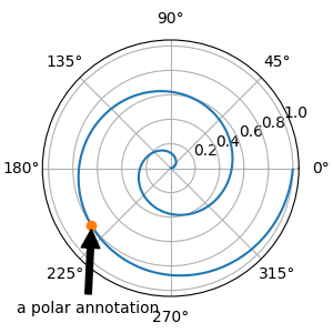
Vous pouvez spécifier le point xy et le xytext dans différentes positions et systèmes de coordonnées, et éventuellement activer une ligne de connexion et marquer le point avec un marqueur. Les annotations fonctionnent également sur les axes polaires.
Dans l'exemple ci-dessous, le point xy est en coordonnées natives ( xycoords par défaut est 'data'). Pour un axe polaire, c'est dans l'espace (thêta, rayon). Le texte de l'exemple est placé dans le système de coordonnées de la figure fractionnaire. Les arguments de mot-clé de texte comme l'alignement horizontal et vertical sont respectés.
fig, ax = plt.subplots(subplot_kw=dict(projection='polar'), figsize=(3, 3))
r = np.arange(0, 1, 0.001)
theta = 2*2*np.pi*r
line, = ax.plot(theta, r)

ind = 800
thisr, thistheta = r[ind], theta[ind]
ax.plot([thistheta], [thisr], 'o')
ax.annotate('a polar annotation',
            xy=(thistheta, thisr),  # theta, radius
            xytext=(0.05, 0.05),    # fraction, fraction
            textcoords='figure fraction',
            arrowprops=dict(facecolor='black', shrink=0.05),
            horizontalalignment='left',
            verticalalignment='bottom')
Text(0.05, 0.05, 'a polar annotation')
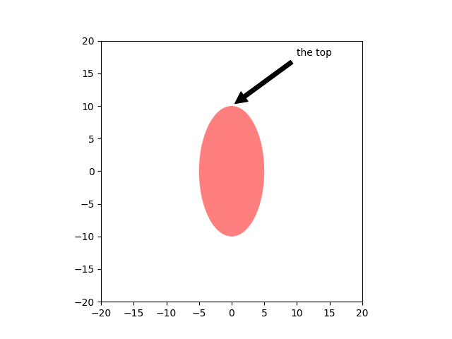
Vous pouvez également utiliser la notation polaire sur un axe cartésien. Ici, le système de coordonnées natif ("data") est cartésien, vous devez donc spécifier les xycoords et textcoords comme "polaire" si vous souhaitez utiliser (thêta, rayon).
el = Ellipse((0, 0), 10, 20, facecolor='r', alpha=0.5)

fig, ax = plt.subplots(subplot_kw=dict(aspect='equal'))
ax.add_artist(el)
el.set_clip_box(ax.bbox)
ax.annotate('the top',
            xy=(np.pi/2., 10.),      # theta, radius
            xytext=(np.pi/3, 20.),   # theta, radius
            xycoords='polar',
            textcoords='polar',
            arrowprops=dict(facecolor='black', shrink=0.05),
            horizontalalignment='left',
            verticalalignment='bottom',
            clip_on=True)  # clip to the axes bounding box

ax.set(xlim=[-20, 20], ylim=[-20, 20])
[(-20.0, 20.0), (-20.0, 20.0)]
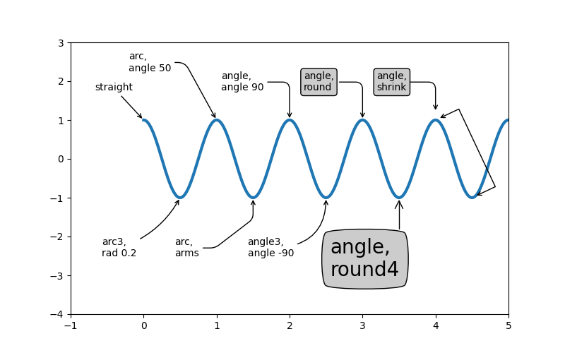
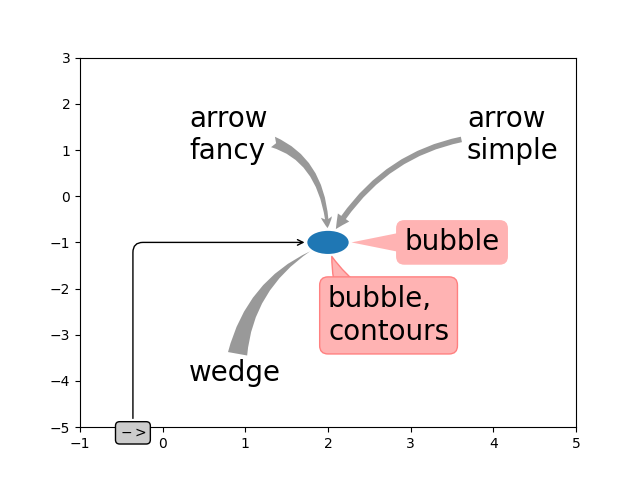
Personnalisation des styles de flèches et de bulles #
La flèche entre xytext et le point d'annotation, ainsi que la bulle qui recouvre le texte d'annotation, sont hautement personnalisables. Vous trouverez ci-dessous quelques options de paramètres ainsi que leur sortie résultante.
fig, ax = plt.subplots(figsize=(8, 5))

t = np.arange(0.0, 5.0, 0.01)
s = np.cos(2*np.pi*t)
line, = ax.plot(t, s, lw=3)

ax.annotate(
    'straight',
    xy=(0, 1), xycoords='data',
    xytext=(-50, 30), textcoords='offset points',
    arrowprops=dict(arrowstyle="->"))
ax.annotate(
    'arc3,\nrad 0.2',
    xy=(0.5, -1), xycoords='data',
    xytext=(-80, -60), textcoords='offset points',
    arrowprops=dict(arrowstyle="->",
                    connectionstyle="arc3,rad=.2"))
ax.annotate(
    'arc,\nangle 50',
    xy=(1., 1), xycoords='data',
    xytext=(-90, 50), textcoords='offset points',
    arrowprops=dict(arrowstyle="->",
                    connectionstyle="arc,angleA=0,armA=50,rad=10"))
ax.annotate(
    'arc,\narms',
    xy=(1.5, -1), xycoords='data',
    xytext=(-80, -60), textcoords='offset points',
    arrowprops=dict(
        arrowstyle="->",
        connectionstyle="arc,angleA=0,armA=40,angleB=-90,armB=30,rad=7"))
ax.annotate(
    'angle,\nangle 90',
    xy=(2., 1), xycoords='data',
    xytext=(-70, 30), textcoords='offset points',
    arrowprops=dict(arrowstyle="->",
                    connectionstyle="angle,angleA=0,angleB=90,rad=10"))
ax.annotate(
    'angle3,\nangle -90',
    xy=(2.5, -1), xycoords='data',
    xytext=(-80, -60), textcoords='offset points',
    arrowprops=dict(arrowstyle="->",
                    connectionstyle="angle3,angleA=0,angleB=-90"))
ax.annotate(
    'angle,\nround',
    xy=(3., 1), xycoords='data',
    xytext=(-60, 30), textcoords='offset points',
    bbox=dict(boxstyle="round", fc="0.8"),
    arrowprops=dict(arrowstyle="->",
                    connectionstyle="angle,angleA=0,angleB=90,rad=10"))
ax.annotate(
    'angle,\nround4',
    xy=(3.5, -1), xycoords='data',
    xytext=(-70, -80), textcoords='offset points',
    size=20,
    bbox=dict(boxstyle="round4,pad=.5", fc="0.8"),
    arrowprops=dict(arrowstyle="->",
                    connectionstyle="angle,angleA=0,angleB=-90,rad=10"))
ax.annotate(
    'angle,\nshrink',
    xy=(4., 1), xycoords='data',
    xytext=(-60, 30), textcoords='offset points',
    bbox=dict(boxstyle="round", fc="0.8"),
    arrowprops=dict(arrowstyle="->",
                    shrinkA=0, shrinkB=10,
                    connectionstyle="angle,angleA=0,angleB=90,rad=10"))
# You can pass an empty string to get only annotation arrows rendered
ax.annotate('', xy=(4., 1.), xycoords='data',
            xytext=(4.5, -1), textcoords='data',
            arrowprops=dict(arrowstyle="<->",
                            connectionstyle="bar",
                            ec="k",
                            shrinkA=5, shrinkB=5))

ax.set(xlim=(-1, 5), ylim=(-4, 3))
[(-1.0, 5.0), (-4.0, 3.0)]
Nous allons créer une autre figure pour qu'elle ne soit pas trop encombrée
fig, ax = plt.subplots()

el = Ellipse((2, -1), 0.5, 0.5)
ax.add_patch(el)

ax.annotate('$->$',
            xy=(2., -1), xycoords='data',
            xytext=(-150, -140), textcoords='offset points',
            bbox=dict(boxstyle="round", fc="0.8"),
            arrowprops=dict(arrowstyle="->",
                            patchB=el,
                            connectionstyle="angle,angleA=90,angleB=0,rad=10"))
ax.annotate('arrow\nfancy',
            xy=(2., -1), xycoords='data',
            xytext=(-100, 60), textcoords='offset points',
            size=20,
            arrowprops=dict(arrowstyle="fancy",
                            fc="0.6", ec="none",
                            patchB=el,
                            connectionstyle="angle3,angleA=0,angleB=-90"))
ax.annotate('arrow\nsimple',
            xy=(2., -1), xycoords='data',
            xytext=(100, 60), textcoords='offset points',
            size=20,
            arrowprops=dict(arrowstyle="simple",
                            fc="0.6", ec="none",
                            patchB=el,
                            connectionstyle="arc3,rad=0.3"))
ax.annotate('wedge',
            xy=(2., -1), xycoords='data',
            xytext=(-100, -100), textcoords='offset points',
            size=20,
            arrowprops=dict(arrowstyle="wedge,tail_width=0.7",
                            fc="0.6", ec="none",
                            patchB=el,
                            connectionstyle="arc3,rad=-0.3"))
ax.annotate('bubble,\ncontours',
            xy=(2., -1), xycoords='data',
            xytext=(0, -70), textcoords='offset points',
            size=20,
            bbox=dict(boxstyle="round",
                      fc=(1.0, 0.7, 0.7),
                      ec=(1., .5, .5)),
            arrowprops=dict(arrowstyle="wedge,tail_width=1.",
                            fc=(1.0, 0.7, 0.7), ec=(1., .5, .5),
                            patchA=None,
                            patchB=el,
                            relpos=(0.2, 0.8),
                            connectionstyle="arc3,rad=-0.1"))
ax.annotate('bubble',
            xy=(2., -1), xycoords='data',
            xytext=(55, 0), textcoords='offset points',
            size=20, va="center",
            bbox=dict(boxstyle="round", fc=(1.0, 0.7, 0.7), ec="none"),
            arrowprops=dict(arrowstyle="wedge,tail_width=1.",
                            fc=(1.0, 0.7, 0.7), ec="none",
                            patchA=None,
                            patchB=el,
                            relpos=(0.2, 0.5)))

ax.set(xlim=(-1, 5), ylim=(-5, 3))
[(-1.0, 5.0), (-5.0, 3.0)]
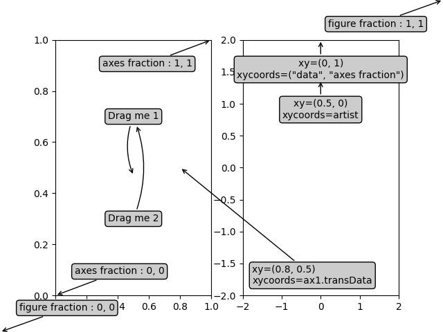
Plus d'exemples de systèmes de coordonnées #
Ci-dessous, nous allons montrer quelques exemples supplémentaires de systèmes de coordonnées et comment l'emplacement des annotations peut être spécifié.
fig, (ax1, ax2) = plt.subplots(1, 2)

bbox_args = dict(boxstyle="round", fc="0.8")
arrow_args = dict(arrowstyle="->")

# Here we'll demonstrate the extents of the coordinate system and how
# we place annotating text.

ax1.annotate('figure fraction : 0, 0', xy=(0, 0), xycoords='figure fraction',
             xytext=(20, 20), textcoords='offset points',
             ha="left", va="bottom",
             bbox=bbox_args,
             arrowprops=arrow_args)

ax1.annotate('figure fraction : 1, 1', xy=(1, 1), xycoords='figure fraction',
             xytext=(-20, -20), textcoords='offset points',
             ha="right", va="top",
             bbox=bbox_args,
             arrowprops=arrow_args)

ax1.annotate('axes fraction : 0, 0', xy=(0, 0), xycoords='axes fraction',
             xytext=(20, 20), textcoords='offset points',
             ha="left", va="bottom",
             bbox=bbox_args,
             arrowprops=arrow_args)

ax1.annotate('axes fraction : 1, 1', xy=(1, 1), xycoords='axes fraction',
             xytext=(-20, -20), textcoords='offset points',
             ha="right", va="top",
             bbox=bbox_args,
             arrowprops=arrow_args)

# It is also possible to generate draggable annotations

an1 = ax1.annotate('Drag me 1', xy=(.5, .7), xycoords='data',
                   ha="center", va="center",
                   bbox=bbox_args)

an2 = ax1.annotate('Drag me 2', xy=(.5, .5), xycoords=an1,
                   xytext=(.5, .3), textcoords='axes fraction',
                   ha="center", va="center",
                   bbox=bbox_args,
                   arrowprops=dict(patchB=an1.get_bbox_patch(),
                                   connectionstyle="arc3,rad=0.2",
                                   **arrow_args))
an1.draggable()
an2.draggable()

an3 = ax1.annotate('', xy=(.5, .5), xycoords=an2,
                   xytext=(.5, .5), textcoords=an1,
                   ha="center", va="center",
                   bbox=bbox_args,
                   arrowprops=dict(patchA=an1.get_bbox_patch(),
                                   patchB=an2.get_bbox_patch(),
                                   connectionstyle="arc3,rad=0.2",
                                   **arrow_args))

# Finally we'll show off some more complex annotation and placement

text = ax2.annotate('xy=(0, 1)\nxycoords=("data", "axes fraction")',
                    xy=(0, 1), xycoords=("data", 'axes fraction'),
                    xytext=(0, -20), textcoords='offset points',
                    ha="center", va="top",
                    bbox=bbox_args,
                    arrowprops=arrow_args)

ax2.annotate('xy=(0.5, 0)\nxycoords=artist',
             xy=(0.5, 0.), xycoords=text,
             xytext=(0, -20), textcoords='offset points',
             ha="center", va="top",
             bbox=bbox_args,
             arrowprops=arrow_args)

ax2.annotate('xy=(0.8, 0.5)\nxycoords=ax1.transData',
             xy=(0.8, 0.5), xycoords=ax1.transData,
             xytext=(10, 10),
             textcoords=OffsetFrom(ax2.bbox, (0, 0), "points"),
             ha="left", va="bottom",
             bbox=bbox_args,
             arrowprops=arrow_args)

ax2.set(xlim=[-2, 2], ylim=[-2, 2])
plt.show()
Durée totale d'exécution du script : (0 minutes 2,463 secondes)