Noter
Cliquez ici pour télécharger l'exemple de code complet
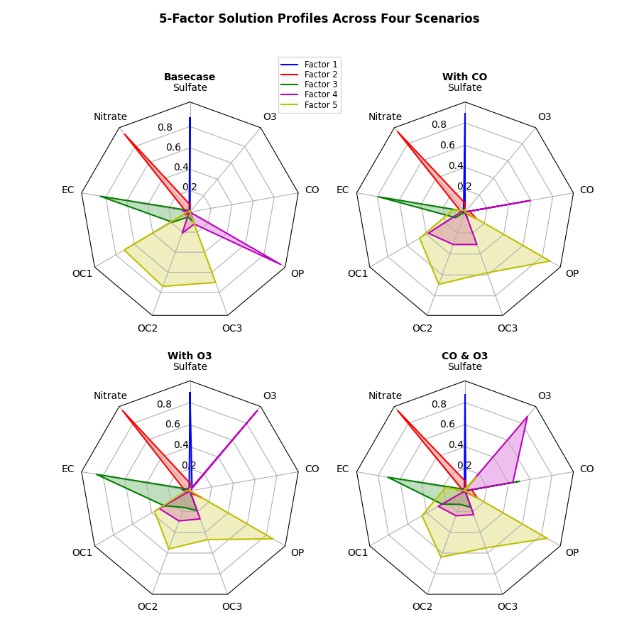
Carte radar (alias carte d'araignée ou étoile) #
Cet exemple crée une carte en radar, également connue sous le nom de carte en toile d'araignée ou en étoile [ 1 ] .
Bien que cet exemple autorise un cadre de 'cercle' ou de 'polygone', les cadres de polygones n'ont pas de quadrillage approprié (les lignes sont des cercles au lieu de polygones). Il est possible d'obtenir une grille de polygones en définissant GRIDLINE_INTERPOLATION_STEPS dans matplotlib.axis sur le nombre de sommets souhaité, mais l'orientation du polygone n'est pas alignée sur les axes radiaux.
import numpy as np

import matplotlib.pyplot as plt
from matplotlib.patches import Circle, RegularPolygon
from matplotlib.path import Path
from matplotlib.projections.polar import PolarAxes
from matplotlib.projections import register_projection
from matplotlib.spines import Spine
from matplotlib.transforms import Affine2D


def radar_factory(num_vars, frame='circle'):
    """
    Create a radar chart with `num_vars` axes.

    This function creates a RadarAxes projection and registers it.

    Parameters
    ----------
    num_vars : int
        Number of variables for radar chart.
    frame : {'circle', 'polygon'}
        Shape of frame surrounding axes.

    """
    # calculate evenly-spaced axis angles
    theta = np.linspace(0, 2*np.pi, num_vars, endpoint=False)

    class RadarTransform(PolarAxes.PolarTransform):

        def transform_path_non_affine(self, path):
            # Paths with non-unit interpolation steps correspond to gridlines,
            # in which case we force interpolation (to defeat PolarTransform's
            # autoconversion to circular arcs).
            if path._interpolation_steps > 1:
                path = path.interpolated(num_vars)
            return Path(self.transform(path.vertices), path.codes)

    class RadarAxes(PolarAxes):

        name = 'radar'
        PolarTransform = RadarTransform

        def __init__(self, *args, **kwargs):
            super().__init__(*args, **kwargs)
            # rotate plot such that the first axis is at the top
            self.set_theta_zero_location('N')

        def fill(self, *args, closed=True, **kwargs):
            """Override fill so that line is closed by default"""
            return super().fill(closed=closed, *args, **kwargs)

        def plot(self, *args, **kwargs):
            """Override plot so that line is closed by default"""
            lines = super().plot(*args, **kwargs)
            for line in lines:
                self._close_line(line)

        def _close_line(self, line):
            x, y = line.get_data()
            # FIXME: markers at x[0], y[0] get doubled-up
            if x[0] != x[-1]:
                x = np.append(x, x[0])
                y = np.append(y, y[0])
                line.set_data(x, y)

        def set_varlabels(self, labels):
            self.set_thetagrids(np.degrees(theta), labels)

        def _gen_axes_patch(self):
            # The Axes patch must be centered at (0.5, 0.5) and of radius 0.5
            # in axes coordinates.
            if frame == 'circle':
                return Circle((0.5, 0.5), 0.5)
            elif frame == 'polygon':
                return RegularPolygon((0.5, 0.5), num_vars,
                                      radius=.5, edgecolor="k")
            else:
                raise ValueError("Unknown value for 'frame': %s" % frame)

        def _gen_axes_spines(self):
            if frame == 'circle':
                return super()._gen_axes_spines()
            elif frame == 'polygon':
                # spine_type must be 'left'/'right'/'top'/'bottom'/'circle'.
                spine = Spine(axes=self,
                              spine_type='circle',
                              path=Path.unit_regular_polygon(num_vars))
                # unit_regular_polygon gives a polygon of radius 1 centered at
                # (0, 0) but we want a polygon of radius 0.5 centered at (0.5,
                # 0.5) in axes coordinates.
                spine.set_transform(Affine2D().scale(.5).translate(.5, .5)
                                    + self.transAxes)
                return {'polar': spine}
            else:
                raise ValueError("Unknown value for 'frame': %s" % frame)

    register_projection(RadarAxes)
    return theta


def example_data():
    # The following data is from the Denver Aerosol Sources and Health study.
    # See doi:10.1016/j.atmosenv.2008.12.017
    #
    # The data are pollution source profile estimates for five modeled
    # pollution sources (e.g., cars, wood-burning, etc) that emit 7-9 chemical
    # species. The radar charts are experimented with here to see if we can
    # nicely visualize how the modeled source profiles change across four
    # scenarios:
    #  1) No gas-phase species present, just seven particulate counts on
    #     Sulfate
    #     Nitrate
    #     Elemental Carbon (EC)
    #     Organic Carbon fraction 1 (OC)
    #     Organic Carbon fraction 2 (OC2)
    #     Organic Carbon fraction 3 (OC3)
    #     Pyrolyzed Organic Carbon (OP)
    #  2)Inclusion of gas-phase specie carbon monoxide (CO)
    #  3)Inclusion of gas-phase specie ozone (O3).
    #  4)Inclusion of both gas-phase species is present...
    data = [
        ['Sulfate', 'Nitrate', 'EC', 'OC1', 'OC2', 'OC3', 'OP', 'CO', 'O3'],
        ('Basecase', [
            [0.88, 0.01, 0.03, 0.03, 0.00, 0.06, 0.01, 0.00, 0.00],
            [0.07, 0.95, 0.04, 0.05, 0.00, 0.02, 0.01, 0.00, 0.00],
            [0.01, 0.02, 0.85, 0.19, 0.05, 0.10, 0.00, 0.00, 0.00],
            [0.02, 0.01, 0.07, 0.01, 0.21, 0.12, 0.98, 0.00, 0.00],
            [0.01, 0.01, 0.02, 0.71, 0.74, 0.70, 0.00, 0.00, 0.00]]),
        ('With CO', [
            [0.88, 0.02, 0.02, 0.02, 0.00, 0.05, 0.00, 0.05, 0.00],
            [0.08, 0.94, 0.04, 0.02, 0.00, 0.01, 0.12, 0.04, 0.00],
            [0.01, 0.01, 0.79, 0.10, 0.00, 0.05, 0.00, 0.31, 0.00],
            [0.00, 0.02, 0.03, 0.38, 0.31, 0.31, 0.00, 0.59, 0.00],
            [0.02, 0.02, 0.11, 0.47, 0.69, 0.58, 0.88, 0.00, 0.00]]),
        ('With O3', [
            [0.89, 0.01, 0.07, 0.00, 0.00, 0.05, 0.00, 0.00, 0.03],
            [0.07, 0.95, 0.05, 0.04, 0.00, 0.02, 0.12, 0.00, 0.00],
            [0.01, 0.02, 0.86, 0.27, 0.16, 0.19, 0.00, 0.00, 0.00],
            [0.01, 0.03, 0.00, 0.32, 0.29, 0.27, 0.00, 0.00, 0.95],
            [0.02, 0.00, 0.03, 0.37, 0.56, 0.47, 0.87, 0.00, 0.00]]),
        ('CO & O3', [
            [0.87, 0.01, 0.08, 0.00, 0.00, 0.04, 0.00, 0.00, 0.01],
            [0.09, 0.95, 0.02, 0.03, 0.00, 0.01, 0.13, 0.06, 0.00],
            [0.01, 0.02, 0.71, 0.24, 0.13, 0.16, 0.00, 0.50, 0.00],
            [0.01, 0.03, 0.00, 0.28, 0.24, 0.23, 0.00, 0.44, 0.88],
            [0.02, 0.00, 0.18, 0.45, 0.64, 0.55, 0.86, 0.00, 0.16]])
    ]
    return data


if __name__ == '__main__':
    N = 9
    theta = radar_factory(N, frame='polygon')

    data = example_data()
    spoke_labels = data.pop(0)

    fig, axs = plt.subplots(figsize=(9, 9), nrows=2, ncols=2,
                            subplot_kw=dict(projection='radar'))
    fig.subplots_adjust(wspace=0.25, hspace=0.20, top=0.85, bottom=0.05)

    colors = ['b', 'r', 'g', 'm', 'y']
    # Plot the four cases from the example data on separate axes
    for ax, (title, case_data) in zip(axs.flat, data):
        ax.set_rgrids([0.2, 0.4, 0.6, 0.8])
        ax.set_title(title, weight='bold', size='medium', position=(0.5, 1.1),
                     horizontalalignment='center', verticalalignment='center')
        for d, color in zip(case_data, colors):
            ax.plot(theta, d, color=color)
            ax.fill(theta, d, facecolor=color, alpha=0.25, label='_nolegend_')
        ax.set_varlabels(spoke_labels)

    # add legend relative to top-left plot
    labels = ('Factor 1', 'Factor 2', 'Factor 3', 'Factor 4', 'Factor 5')
    legend = axs[0, 0].legend(labels, loc=(0.9, .95),
                              labelspacing=0.1, fontsize='small')

    fig.text(0.5, 0.965, '5-Factor Solution Profiles Across Four Scenarios',
             horizontalalignment='center', color='black', weight='bold',
             size='large')

    plt.show()
Références
L'utilisation des fonctions, méthodes, classes et modules suivants est illustrée dans cet exemple :
Durée totale d'exécution du script : (0 minutes 1,611 secondes)