Démo PSD

Tracé de la densité spectrale de puissance (PSD) dans Matplotlib.

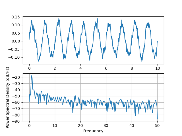
La PSD est un tracé courant dans le domaine du traitement du signal. NumPy possède de nombreuses bibliothèques utiles pour calculer un PSD. Ci-dessous, nous démontrons quelques exemples de la façon dont cela peut être accompli et visualisé avec Matplotlib.

import matplotlib.pyplot as plt
import numpy as np
import matplotlib.mlab as mlab

# Fixing random state for reproducibility
np.random.seed(19680801)

dt = 0.01
t = np.arange(0, 10, dt)
nse = np.random.randn(len(t))
r = np.exp(-t / 0.05)

cnse = np.convolve(nse, r) * dt
cnse = cnse[:len(t)]
s = 0.1 * np.sin(2 * np.pi * t) + cnse

fig, (ax0, ax1) = plt.subplots(2, 1)
ax0.plot(t, s)
ax1.psd(s, 512, 1 / dt)

plt.show()

Comparez cela avec le code Matlab équivalent pour accomplir la même chose :

dt = 0.01;
t = [0:dt:10];
nse = randn(size(t));
r = exp(-t/0.05);
cnse = conv(nse, r)*dt;
cnse = cnse(1:length(t));
s = 0.1*sin(2*pi*t) + cnse;

subplot(211)
plot(t, s)
subplot(212)
psd(s, 512, 1/dt)

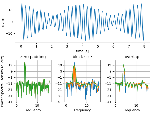
Ci-dessous, nous allons montrer un exemple légèrement plus complexe qui montre comment le rembourrage affecte le PSD résultant.

dt = np.pi / 100.
fs = 1. / dt
t = np.arange(0, 8, dt)
y = 10. * np.sin(2 * np.pi * 4 * t) + 5. * np.sin(2 * np.pi * 4.25 * t)
y = y + np.random.randn(*t.shape)

# Plot the raw time series
fig, axs = plt.subplot_mosaic([
    ['signal', 'signal', 'signal'],
    ['zero padding', 'block size', 'overlap'],
], layout='constrained')

axs['signal'].plot(t, y)
axs['signal'].set_xlabel('time [s]')
axs['signal'].set_ylabel('signal')

# Plot the PSD with different amounts of zero padding. This uses the entire
# time series at once
axs['zero padding'].psd(y, NFFT=len(t), pad_to=len(t), Fs=fs)
axs['zero padding'].psd(y, NFFT=len(t), pad_to=len(t) * 2, Fs=fs)
axs['zero padding'].psd(y, NFFT=len(t), pad_to=len(t) * 4, Fs=fs)

# Plot the PSD with different block sizes, Zero pad to the length of the
# original data sequence.
axs['block size'].psd(y, NFFT=len(t), pad_to=len(t), Fs=fs)
axs['block size'].psd(y, NFFT=len(t) // 2, pad_to=len(t), Fs=fs)
axs['block size'].psd(y, NFFT=len(t) // 4, pad_to=len(t), Fs=fs)
axs['block size'].set_ylabel('')

# Plot the PSD with different amounts of overlap between blocks
axs['overlap'].psd(y, NFFT=len(t) // 2, pad_to=len(t), noverlap=0, Fs=fs)
axs['overlap'].psd(y, NFFT=len(t) // 2, pad_to=len(t),
                   noverlap=int(0.025 * len(t)), Fs=fs)
axs['overlap'].psd(y, NFFT=len(t) // 2, pad_to=len(t),
                   noverlap=int(0.1 * len(t)), Fs=fs)
axs['overlap'].set_ylabel('')
axs['overlap'].set_title('overlap')

for title, ax in axs.items():
    if title == 'signal':
        continue

    ax.set_title(title)
    ax.sharex(axs['zero padding'])
    ax.sharey(axs['zero padding'])

plt.show()

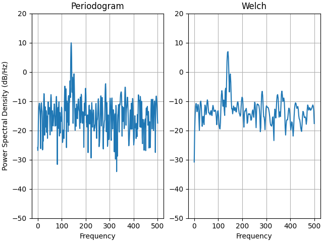
Il s'agit d'une version portée d'un exemple MATLAB de la boîte à outils de traitement du signal qui a montré une certaine différence à un moment donné entre la mise à l'échelle de Matplotlib et MATLAB du PSD.

fs = 1000
t = np.linspace(0, 0.3, 301)
A = np.array([2, 8]).reshape(-1, 1)
f = np.array([150, 140]).reshape(-1, 1)
xn = (A * np.sin(2 * np.pi * f * t)).sum(axis=0)
xn += 5 * np.random.randn(*t.shape)

fig, (ax0, ax1) = plt.subplots(ncols=2, constrained_layout=True)

yticks = np.arange(-50, 30, 10)
yrange = (yticks[0], yticks[-1])
xticks = np.arange(0, 550, 100)

ax0.psd(xn, NFFT=301, Fs=fs, window=mlab.window_none, pad_to=1024,
        scale_by_freq=True)
ax0.set_title('Periodogram')
ax0.set_yticks(yticks)
ax0.set_xticks(xticks)
ax0.grid(True)
ax0.set_ylim(yrange)

ax1.psd(xn, NFFT=150, Fs=fs, window=mlab.window_none, pad_to=512, noverlap=75,
        scale_by_freq=True)
ax1.set_title('Welch')
ax1.set_xticks(xticks)
ax1.set_yticks(yticks)
ax1.set_ylabel('')  # overwrite the y-label added by `psd`
ax1.grid(True)
ax1.set_ylim(yrange)

plt.show()

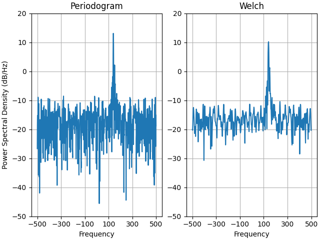
Il s'agit d'une version portée d'un exemple MATLAB de la boîte à outils de traitement du signal qui a montré une certaine différence à un moment donné entre la mise à l'échelle de Matplotlib et MATLAB du PSD.

Il utilise un signal complexe afin que nous puissions voir que les PSD complexes fonctionnent correctement.

prng = np.random.RandomState(19680801)  # to ensure reproducibility

fs = 1000
t = np.linspace(0, 0.3, 301)
A = np.array([2, 8]).reshape(-1, 1)
f = np.array([150, 140]).reshape(-1, 1)
xn = (A * np.exp(2j * np.pi * f * t)).sum(axis=0) + 5 * prng.randn(*t.shape)

fig, (ax0, ax1) = plt.subplots(ncols=2, constrained_layout=True)

yticks = np.arange(-50, 30, 10)
yrange = (yticks[0], yticks[-1])
xticks = np.arange(-500, 550, 200)

ax0.psd(xn, NFFT=301, Fs=fs, window=mlab.window_none, pad_to=1024,
        scale_by_freq=True)
ax0.set_title('Periodogram')
ax0.set_yticks(yticks)
ax0.set_xticks(xticks)
ax0.grid(True)
ax0.set_ylim(yrange)

ax1.psd(xn, NFFT=150, Fs=fs, window=mlab.window_none, pad_to=512, noverlap=75,
        scale_by_freq=True)
ax1.set_title('Welch')
ax1.set_xticks(xticks)
ax1.set_yticks(yticks)
ax1.set_ylabel('')  # overwrite the y-label added by `psd`
ax1.grid(True)
ax1.set_ylim(yrange)

plt.show()