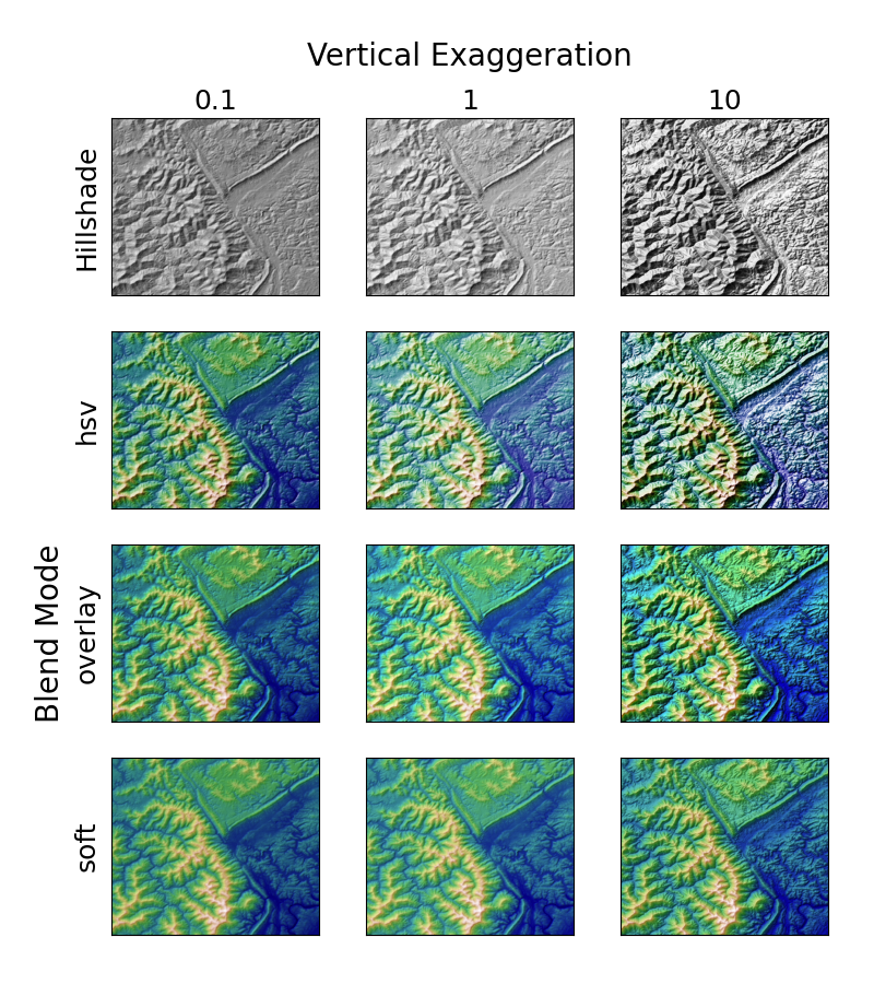
Ombrage topographique

Démontre l'effet visuel de la variation du mode de fusion et de l'exagération verticale sur les tracés "ombrés".

Notez que les modes de fusion "overlay" et "soft" fonctionnent bien pour les surfaces complexes telles que cet exemple, tandis que le mode de fusion "hsv" par défaut fonctionne mieux pour les surfaces lisses telles que de nombreuses fonctions mathématiques.

Dans la plupart des cas, l'ombrage est utilisé uniquement à des fins visuelles, et dx / dy peut être ignoré en toute sécurité. Dans ce cas, vous pouvez modifier vert_exag (exagération verticale) par essais et erreurs pour donner l'effet visuel souhaité. Cependant, cet exemple montre comment utiliser les arguments de mot-clé dx et dy pour s'assurer que le paramètre vert_exag est la véritable exagération verticale.

import numpy as np
import matplotlib.pyplot as plt
from matplotlib.cbook import get_sample_data
from matplotlib.colors import LightSource


dem = get_sample_data('jacksboro_fault_dem.npz', np_load=True)
z = dem['elevation']
# -- Optional dx and dy for accurate vertical exaggeration --------------------
# If you need topographically accurate vertical exaggeration, or you don't want
# to guess at what *vert_exag* should be, you'll need to specify the cellsize
# of the grid (i.e. the *dx* and *dy* parameters).  Otherwise, any *vert_exag*
# value you specify will be relative to the grid spacing of your input data
# (in other words, *dx* and *dy* default to 1.0, and *vert_exag* is calculated
# relative to those parameters).  Similarly, *dx* and *dy* are assumed to be in
# the same units as your input z-values.  Therefore, we'll need to convert the
# given dx and dy from decimal degrees to meters.
dx, dy = dem['dx'], dem['dy']
dy = 111200 * dy
dx = 111200 * dx * np.cos(np.radians(dem['ymin']))
# -----------------------------------------------------------------------------

# Shade from the northwest, with the sun 45 degrees from horizontal
ls = LightSource(azdeg=315, altdeg=45)
cmap = plt.cm.gist_earth

fig, axs = plt.subplots(nrows=4, ncols=3, figsize=(8, 9))
plt.setp(axs.flat, xticks=[], yticks=[])

# Vary vertical exaggeration and blend mode and plot all combinations
for col, ve in zip(axs.T, [0.1, 1, 10]):
    # Show the hillshade intensity image in the first row
    col[0].imshow(ls.hillshade(z, vert_exag=ve, dx=dx, dy=dy), cmap='gray')

    # Place hillshaded plots with different blend modes in the rest of the rows
    for ax, mode in zip(col[1:], ['hsv', 'overlay', 'soft']):
        rgb = ls.shade(z, cmap=cmap, blend_mode=mode,
                       vert_exag=ve, dx=dx, dy=dy)
        ax.imshow(rgb)

# Label rows and columns
for ax, ve in zip(axs[0], [0.1, 1, 10]):
    ax.set_title('{0}'.format(ve), size=18)
for ax, mode in zip(axs[:, 0], ['Hillshade', 'hsv', 'overlay', 'soft']):
    ax.set_ylabel(mode, size=18)

# Group labels...
axs[0, 1].annotate('Vertical Exaggeration', (0.5, 1), xytext=(0, 30),
                   textcoords='offset points', xycoords='axes fraction',
                   ha='center', va='bottom', size=20)
axs[2, 0].annotate('Blend Mode', (0, 0.5), xytext=(-30, 0),
                   textcoords='offset points', xycoords='axes fraction',
                   ha='right', va='center', size=20, rotation=90)
fig.subplots_adjust(bottom=0.05, right=0.95)

plt.show()