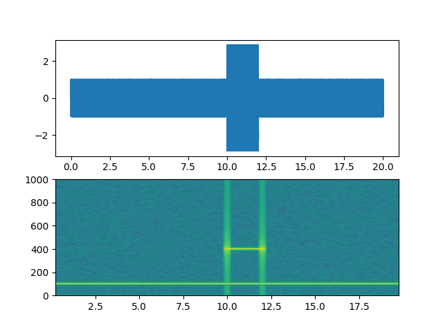
Démonstration du spectrogramme

Démo d'un tracé de spectrogramme ( specgram).

import matplotlib.pyplot as plt
import numpy as np

# Fixing random state for reproducibility
np.random.seed(19680801)

dt = 0.0005
t = np.arange(0.0, 20.0, dt)
s1 = np.sin(2 * np.pi * 100 * t)
s2 = 2 * np.sin(2 * np.pi * 400 * t)

# create a transient "chirp"
s2[t <= 10] = s2[12 <= t] = 0

# add some noise into the mix
nse = 0.01 * np.random.random(size=len(t))

x = s1 + s2 + nse  # the signal
NFFT = 1024  # the length of the windowing segments
Fs = int(1.0 / dt)  # the sampling frequency

fig, (ax1, ax2) = plt.subplots(nrows=2)
ax1.plot(t, x)
Pxx, freqs, bins, im = ax2.specgram(x, NFFT=NFFT, Fs=Fs, noverlap=900)
# The `specgram` method returns 4 objects. They are:
# - Pxx: the periodogram
# - freqs: the frequency vector
# - bins: the centers of the time bins
# - im: the .image.AxesImage instance representing the data in the plot
plt.show()

Références

L'utilisation des fonctions, méthodes, classes et modules suivants est illustrée dans cet exemple :

• matplotlib.axes.Axes.specgram/matplotlib.pyplot.specgram